State-Space Control of an Inverted Pendulum

Problem Setup

In the previous post, I gave a walk-through how we could design a controller for the inverted pendulum using frequency domain techniques. In this post, we will the design of a controller for the same system using state-space methods. Recall the linearized equations of motion of the inverted pendulum about the upright position:

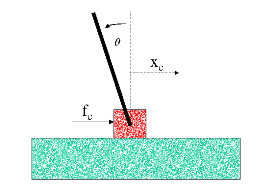
\[\begin{bmatrix} M_{c}+M_{R}+I_{mot}\frac{k^2}{R^2} & -\frac{1}{2}M_{R}L \\ -1 & \frac{2}{3}L \\ \end{bmatrix} \begin{bmatrix} \ddot{x}_{c} \\ \ddot{\theta} \end{bmatrix} - \begin{bmatrix} 0 \\ g \end{bmatrix} \theta = \begin{bmatrix} 1 \\ 0 \end{bmatrix} f_{c}\]

where \(x_{c}\) is the position of the cart, \(\theta\) is the angle the pendulum makes with the vertical axis, \(M_{c}\) is the mass of the cart, \(M_{R}\) is the mass of the pendulum rod, \(L\) is the length of the pendulum rod, and \(I_{rot}\) is the motor’s moment of inertia. The input into the system is \(f_{c}=\alpha_{1}V+\alpha_{2}\dot{x}_{c}\), where we get to control the voltage supplied to the cart’s motor, \(V\).

For ease of notation, let us define the following:

\[H\triangleq\begin{bmatrix} M_{c}+M_{R}+I_{mot}\frac{k^2}{R^2} & -\frac{1}{2}M_{R}L \\ -1 & \frac{2}{3}L \\ \end{bmatrix}\]

Then we can rewrite the linearized equations of motion in state-space representation as the following:

\[\begin{bmatrix} \dot{x}_{c} \\ \dot{\theta} \\ \ddot{x}_{c} \\ \ddot{\theta} \end{bmatrix} = \begin{bmatrix} 0 & 0 & 1 & 0 \\ 0 & 0 & 0 & 1 \\ \begin{bmatrix} 0 \\ 0 \end{bmatrix} & H^{-1}\begin{bmatrix} 0 \\ g \end{bmatrix} & H^{-1}\begin{bmatrix} \alpha_{2} \\ 0 \end{bmatrix} & \begin{bmatrix} 0 \\ 0 \end{bmatrix} \end{bmatrix} \begin{bmatrix} {x}_{c} \\ \theta \\ \dot{x_{c}} \\ \dot{\theta} \end{bmatrix} +H^{-1}\begin{bmatrix} \alpha_{1} \\ 0 \end{bmatrix}u\]

This tells us the \(A\) and \(B\) matrices:

\[A= \begin{bmatrix} 0 & 0 & 1 & 0 \\ 0 & 0 & 0 & 1 \\ \begin{bmatrix} 0 \\ 0 \end{bmatrix} & H^{-1}\begin{bmatrix} 0 \\ g \end{bmatrix} & H^{-1}\begin{bmatrix} \alpha_{2} \\ 0 \end{bmatrix} & \begin{bmatrix} 0 \\ 0 \end{bmatrix} \end{bmatrix}\] \[B= H^{-1}\begin{bmatrix} \alpha_{1} \\ 0 \end{bmatrix}\]

We will design two controllers: (1) a SISO (single-input single-output) controller and (2) a SIMO (single-input multiple-output) controller. For controller (1), we have a scalar output \(y=x_{c}-\frac{2}{3}L\theta\) that lumps together the two measurements \(x_{c}\) and \(\theta\). Note that this output is basically the x position of the 1/3 point of the rod from the base. For controller (2), the output is a 2 by 1 vector, \(\begin{bmatrix} x_{c} \\ \theta \end{bmatrix}\). Consequently, the two controllers will have difference C matrices. For controller (1),

\[C_{SISO}= \begin{bmatrix} 1 & -\frac{2}{3}L & 0 & 0 \end{bmatrix}\]

For controller (2),

\[C_{SIMO}= \begin{bmatrix} 1 & 0 & 0 & 0 \\ 0 & 1 & 0 & 0 \end{bmatrix}\]

Controller Design

In both cases (SISO and SIMO system), we do not have access to the full state. That is, we need to implement an observer (i.e. state estimator) to estimate the state based on our measurements \(y\). The block diagram that implements this looks like the following:

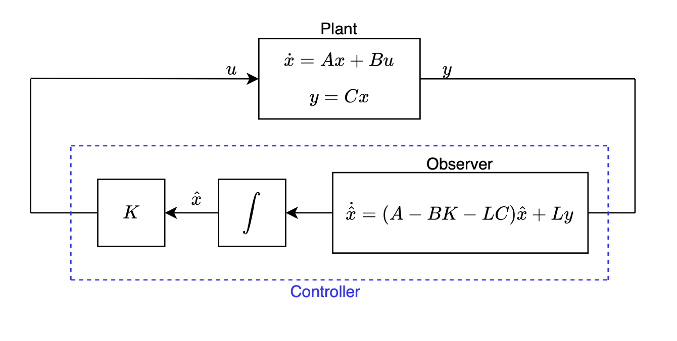
Or equivalently,

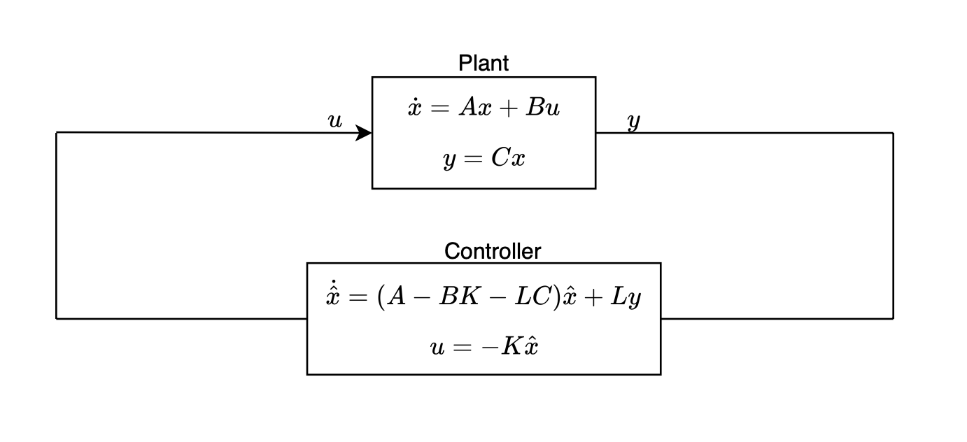
This block diagram lets us write the following four equations:

\[\dot{x}=Ax+Bu\] \[y=Cx\] \[\dot{\hat{x}}=(A-BK-LC)\hat{x}+Ly\] \[u=-K\hat{x}\]

Substituting the fourth equation into the first equation and substituting the second equation into the third equation gives us:

\[\dot{x}=Ax-BK\hat{x}\] \[\dot{\hat{x}}=(A-BK-LC)\hat{x}+LCx\]

Furthermore, let us define the error \(e\) as \(e=x-\hat{x}\) and define a new state vector \(q\):

\[q= \begin{bmatrix} x \\ e \end{bmatrix}\]

This gives us a new state-space representation:

\[\dot{q}= \begin{bmatrix} \dot{x} \\ \dot{e} \end{bmatrix}= \begin{bmatrix} A-BK & BK \\ 0 & A-LC \end{bmatrix} \begin{bmatrix} x \\ e \end{bmatrix}\]

The eigenvalues of the new \(A\) matrix is the union of the eigenvalues of \(A-BK\) and the eigenvalues of \(A-LC\). To drive the state \(x\) to zero (or more precisely, the zero vector), we must choose \(K\) such that the eigenvalues of \(A-BK\) are in the LHP and to drive the error \(e\) to zero, we must choose \(L\) such that the eigenvalues of \(A-LC\) are in the LHP. The fact that we can design \(K\) and \(L\) separately (i.e. design \(K\) as if full-state is available for feedback) is referred to as the separation principle.

The only thing left to do now is to choose where to place the eigenvalues of \(A-BK\) and \(A-LC\). As a guideline for choosing \(K\) and \(L\), we were given the following requirements:

The closed-loop control system is stable
Disturbance rejection settling time \(T^{10\%}_{s} < 2s\)
The damping ratio \(\zeta\) is at least \(1/\sqrt{2}\) in order to avoid oscillatory behavior
The eigenvalues of your observer should be around 3 times the real part of the eigenvalues of your controller
\(\vert \lambda \vert <80\) for all eigenvalues

Determining where exactly where should place the eigenvalues was largely by trial-and-error. While placing the eigenvalues farther into the LHP leads to faster convergence for both the state and the error, this can be problematic as it will request too large of a control input from the actuator (i.e. motor). This is in fact what I observed in practice. Initially, for both the SISO and SIMO controllers, I chose all four eigenvalues of \(A-BK\) to have real parts less than (i.e. more negative than) -20. Even though simulating the system with these eigenvalues satisfied the disturbance rejection settling time, because the real part of the eigenvalues quite large, this led to a lot of side-to-side jittery motion in the cart which made it hard to balance the pendulum. I noticed this and incrementally made the magnitude of the eigenvalues smaller, eventually obtaining a stable closed-loop system with eigenvalues \(\lambda_{1,2}=-7\pm0.5i\), \(\lambda_{3}=-6\), \(\lambda_{4}=-5.9\) for the SISO controller and \(\lambda_{1}=-10\), \(\lambda_{2}=-9.5\), \(\lambda_{3}=-10.5\), \(\lambda_{4}=-11\) for the SIMO controller. Here is the simulated response of the SISO and SIMO systems in response to an initial condition of \(x_{0} =[0 \; 0.147 \; 0 \; 0 \; 0 \; 0 \; 0 \; 0]'\) (i.e. initial angle of 8.42 degrees and zero initial error) simulated using MATLAB:

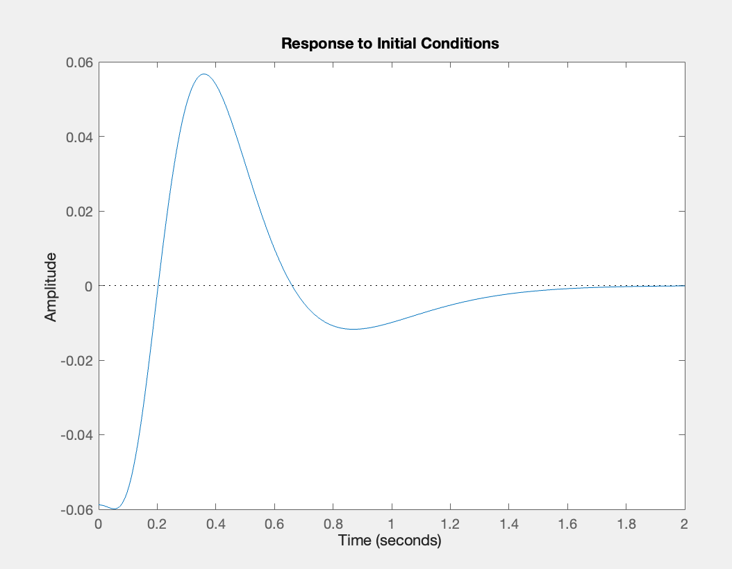
Simulation of SISO system in response to nonzero initial angle

Note: the y-axis is the output, which in the case of the SISO system, is \(y=x_{c}-\frac{2}{3}L\theta\).

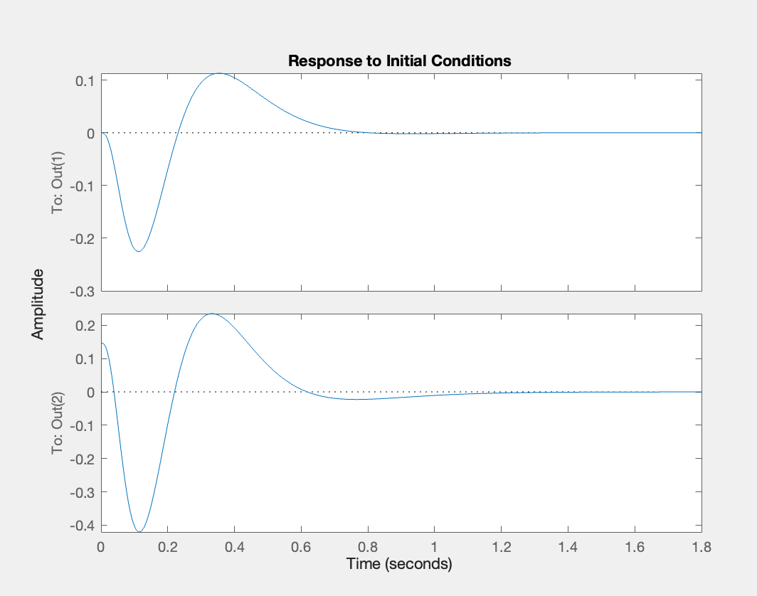
Simulation of SIMO system in response to nonzero initial angle

Note: the SIMO system has 2 outputs (\(x_{c}\) and \(\theta\)); the top graph corresponds to response of \(x_{c}\) and the bottom graph corresponds to response of \(\theta\).

You can see that in both cases, the settling time is less than 2 seconds.

The following is a video that shows the SISO controller successfully stabilizing the system:

The following is a video that shows the SIMO controller successfully stabilizing the system:

Comparison between the SISO and SIMO Controllers

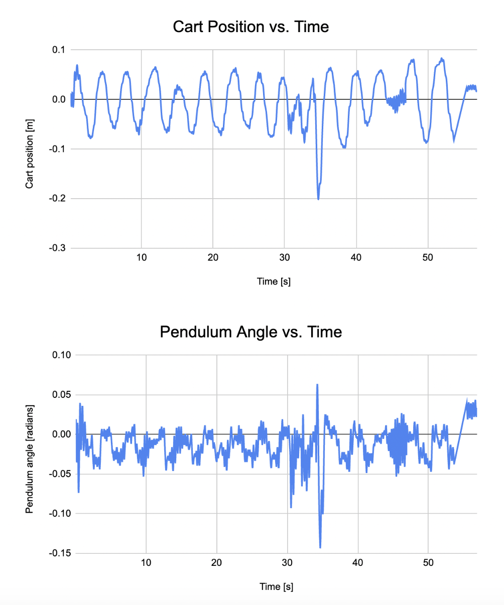
Next, let us compare the performance of the two controllers. The following are the cart position and pendulum angle versus time plots for the SISO controller with roughly zero angle initial conditions:

The following are the cart position and pendulum angle versus time plots for the SIMO controller with roughly zero angle initial conditions:

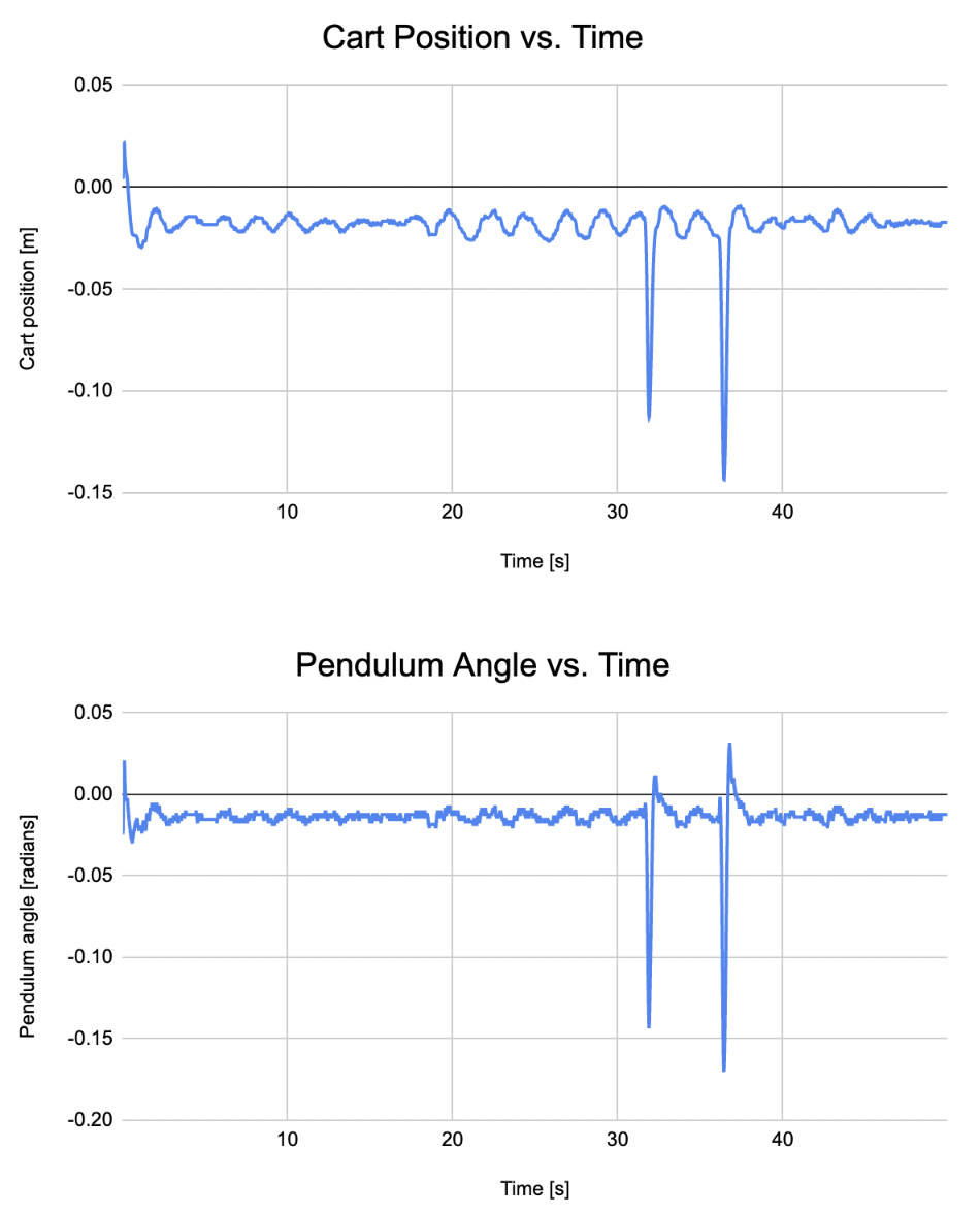
Any spikes in the plots correspond to when we tried to disturb the system by giving the pendulum a little push.In both cases, the controller was able to reject the disturbance input (i.e. bring the system back to equilibrium after the disturbance input was applied).

We can see that the SIMO controller is significantly more stable than the SISO controller. As seen in the plots above, both the cart position and pendulum oscillate considerably for the SISO controller while the cart position and pendulum angle stay very close to zero without much oscillation. This is presumably because the SIMO controller has a greater ability to estimate the state with two outputs rather, leading to faster error convergence in the observer. However, this improvement in controller performance comes with a trade-off: incorporating additional sensors boosts control performance but also escalates costs. Thus, striking the right balance between the two is crucial in the engineering design of any system.

Another thing worth noting is that we chose the gain matrix \(K\) and the observer gain matrix rather arbitrarily by trial and error until they satisfied the required disturbance rejection settling time and damping ratio (a method called pole placement). A more systematic approach to computing \(K\) and \(L\) would be to implement a LQG (Linear Quadratic Gaussian) controller, which is a combination of LQR (Linear Quadratic Control) and Kalman filter. In LQG, instead of choosing \(K\) directly, you choose the penalty weights for state deviation and control input, which are more intuitive than choosing \(K\) directly via pole placement. As for \(L\), LQG finds the optimal observer matrix \(L\) that minimizes the error covariance of the state estimate, eliminating the need for any arbitrary guessing. The separation principle still holds - you can still design \(K\) as if it was a LQR problem by itself and design \(L\) as if it was a Kalman filter problem by itself.